About.
JULES has over a hundred internal parameters representing the environmental sensitivities of the various land-surface types and PFTs within the model. In general these parameters are chosen to represent measurable “realworld” quantities (e.g. aerodynamic roughness length, surface albedo, plant root depth).
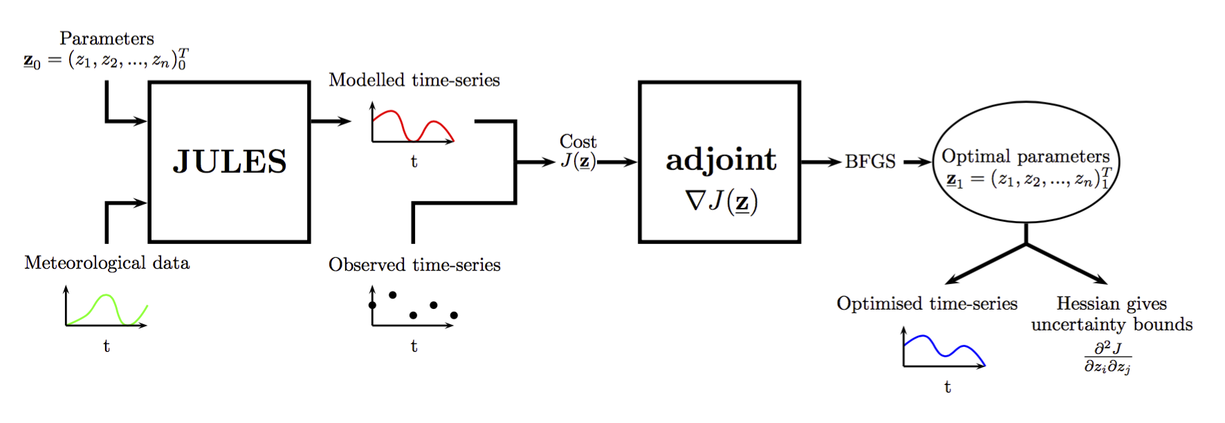
Data assimilation is the act of incorprating observations into a model. By changing the internal parameters of the model, the model output can be made to more closely resemble the observed time-series. The optimal set of parameters is one that minimises the difference between the model output and the observed time-series the most. In order to minimse this difference, the 'adjoint' of JULES is used. This is a complex piece of code, derived by automatic differentiation, which enables efficient and objective calibration against observations. The adjoint is central to the adJULES parameter estimation system, hence the name.
Example
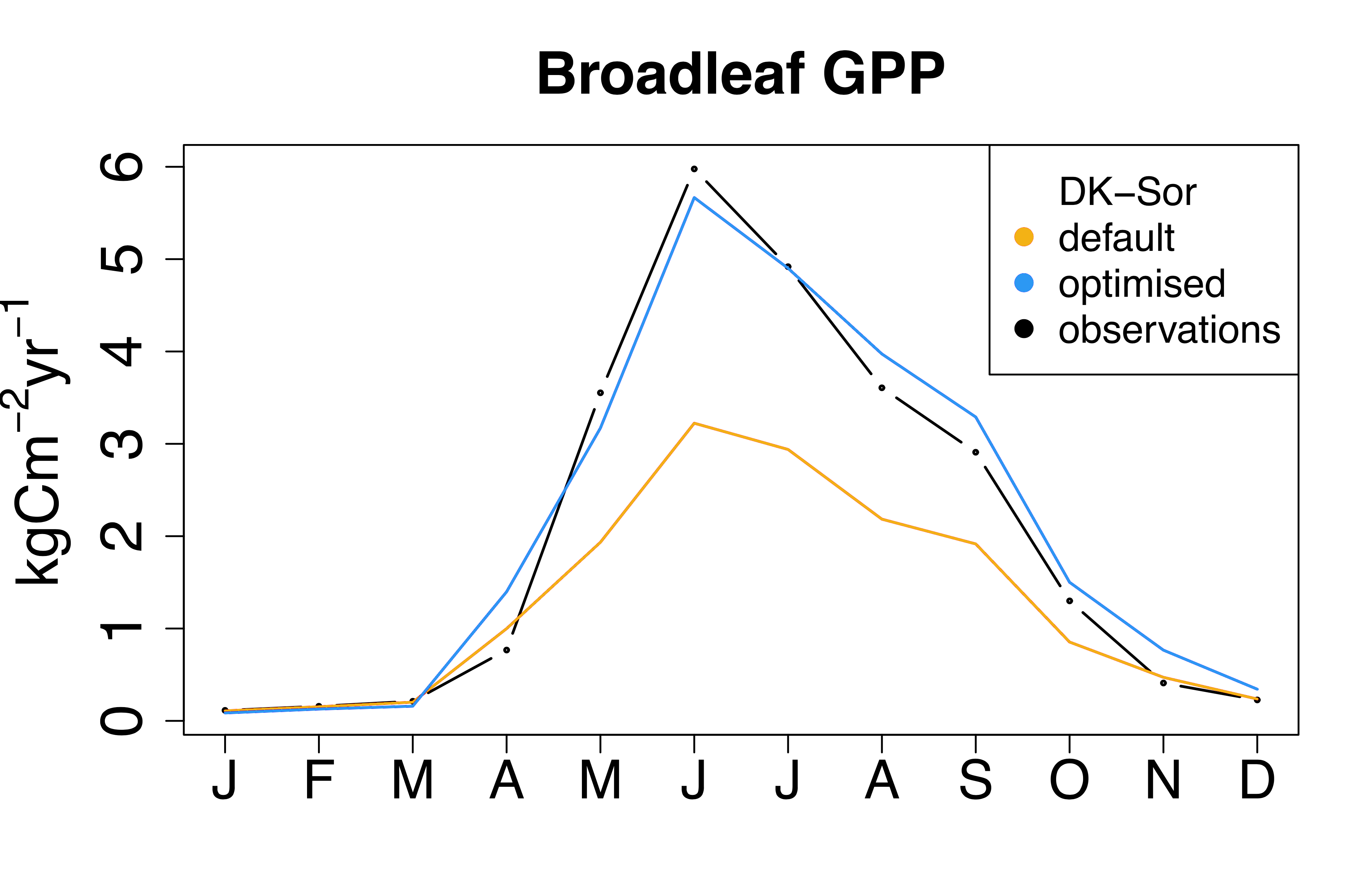
These figures show the time-series of latent heat (left) and a photosynthesis flux called GPP (right) at a measurement site in Denmark (DK-Sor). The observations (black) are compared to JULES runs using default parameters (orange) and optimised parameters (blue). The optimised run can be seen to be much closer to the observations than the default JULES run.

Theoretical Background
For a given subset of internal parameters ($\mathbf{z}$), JULES generates a modelled time-series. A misfit or cost function which measures the mismatch between this time-series and the observations is created. The function also includes a term which measures the mismatch between the parameter values ($\mathbf{z}$) and the initial parameter values ($\mathbf{z}_0$). Finally the function is weighted by the prior error covariance matrixes on observations $\mathbf{R}$ and paramters $\mathbf{B}$. This function is minimised with respect to the parameters in order to find the best fit. $$J(\mathbf{z};\mathbf{z}_0) = \frac{1}{2}\left[\sum_t (\mathbf{m}_{t}(\mathbf{z})-\mathbf{o}_{t})^{T}\mathbf{R}^{-1} (\mathbf{m}_{t}(\mathbf{z})-\mathbf{o}_{t}) + (\mathbf{z}-\mathbf{z}_{0})^{T}\mathbf{B}^{-1}(\mathbf{z}-\mathbf{z}_0)\right]$$ There are several ways this cost function could be minimised. The adJULES system uses what is called a gradient descent method. Gradient descent methods utilise the first-derivative of the cost to identicate which direction in parameter shape minimises the function. The second-derivative of the cost (called the Hessian) can also be used to map the curvature of parameter space and therefore show which direction minimises the function the fastest. Gradient descent methods iteratively minimise the cost function using this information until the optimimum (i.e. gradient $\approx$ 0) is reached or the bounds of the function are hit. The iterative algorthim currently used in the adJULES system is call the BFGS.
The first and second derivative of the cost function are calculated analytically using the adjoint of the JULES model. This information can also be used at the optimum to generate uncertainties associated to each parameter. If curvature of parameter space at the optimum has steep sides, there is low uncertainty associated to the parameter as moving it will significantly increase the cost. If the sides are flat, there is high uncertainty associated to the parameter.

Data
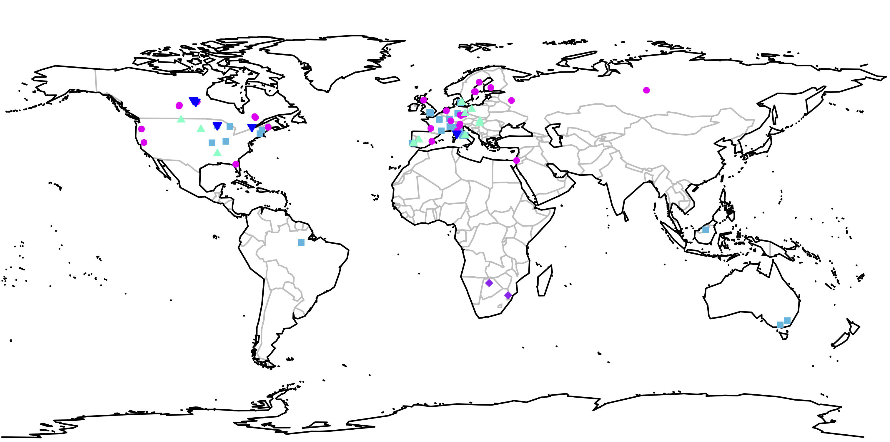
FluxNet data are currently integrated in the adJULES distribution. These provide driving data for JULES and observations against which to calibrate the model.
Currently, the adJULES system uses in situ data from individual or multiple sites to calibrate these parameters. New data sources such as satellite products are expected to be integrated into the system soon.
Emergent constraint
One of the key model parameters was found by Booth et al. (2012) to dominate the spread of climate-carbon cycle feedbacks on JULES. This parameter, $T_{opt}$, corresponding to the optimal temperature for non-light-limited photosynthesis for broadleaf forests, was found to be anti-correlated with net CO2 change by 2100 ($\Delta$CO$_2$) - i.e., if the optimal temperature for photosynthesis for broadleaf trees is high, more CO$_2$ is predicted to be removed from the atmosphere through increased CO$_2$ fertilisation. Using linear regression, we can exploit this relationship to calculate a probability distribution function (PDF) for the distribution of $\Delta\text{CO}_2$ given $T_{opt}$, i.e., $P\{\Delta\text{CO}_2|T_{opt}\}$. The contours of equal probability density around the best-fit linear regression follow a Gaussian probability density $$ P\{\Delta\text{CO}_2|T_{opt}\} = \frac{1}{\sqrt{2\pi\sigma^2_f}}\exp\left\{-\frac{(\Delta\text{CO}_2-f(T_{opt}))^2}{2\sigma_f^2}\right\}$$ where $f$ is the function describing the linear regression between $\Delta\text{CO}_2$ and $T_{opt}$, and $\sigma_f$ is the "prediction error" of the regression.
When combined with $P(T_{opt})$ found by adJULES, and following the method used by Cox et al. (2018) we can calculate the PDF for $\Delta$CO$_2$ by numerically integrating over the product of two PDFs, $P\{\Delta\text{CO}_2|T_{opt}\}$ and $P(T_{opt})$: \begin{equation} P(\Delta\text{CO}_2) = \int^{\infty}_{-\infty} P\{\Delta\text{CO}_2|T_{opt}\}P(T_{opt})dT_{opt}. \end{equation}
