CLARION.

Identifying parameters

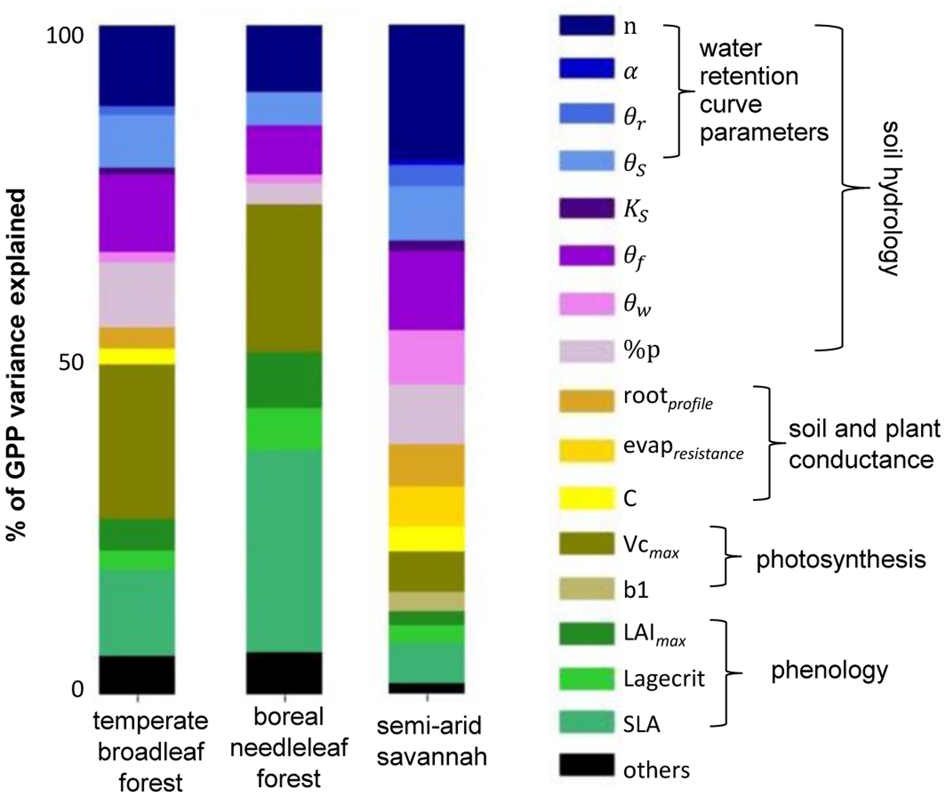
Sensitivity analyses are an important first step in any calibration exercise to identify the key internal parameters which have the most impact on the given model output. This is because; i) DA techniques can be costly and scale with the number of parameters used in the optimisation, and ii) attempting to calibrate an excessive number of parameters can lead to overfitting, and a severe degradation in model performance when the model is used in predictive mode. To carry-out a parameter-sensitivity study, the model is run in forward mode with many sets of feasible parameter values. Using specialised algorithms, it is then possible to calculate how much each parameter contributes to the variances of a modelled output. Below is an example using the Sobol algorithm, we are able to demonstrate the relative importance of key model parameters for simulated gross primary productivity (GPP) at three contrasting locations. At the temperate site (a), GPP is mostly controlled by maximum carboxylation rate (Vcmax). At the boreal site (b), where light can be limiting, parameters controlling the shape of the leaf gain importance (e.g. SLA - specific leaf area). At the semi-arid site (c), where plants can become water-stressed, parameters controlling the amount of SSM dominate (n - determines the shape of the Van Genuchten water retention curve).

Exploring Bayesian techniques and novel datasets for calibration

Bayesian techniques

Calibration of land surface models is of vital importance to ensure accurate predictions of the land surface under climate change. However, these models are complex and calibrations at global scale face a number of challenges. There is also a high degree of parameter uncertainty that needs to be quantifying. Fortunetely, new methods have been emerging and the rise of the machine learning has led to more ensemble based methods to be used. One approach is the so-called history matching method (HM) to tune LSM parameters. This is a different approach which asks not what is the best set to use but, rather, what parameters can we rule out: what regions of parameter space lead to model outputs being "too far" from observations? To do this, HM uses an implausibility function, based on metrics chosen to assess the performance of the model, to rule-out unlikely parameters. HM commonly uses an iterative approach known as iterative refocusing to reduce parameter space, leaving the least unlikely parameter values - the not-ruled out yet (NROY) space. This is a more conservative approach to calibration, primarily used for uncertainty quantification, helping to identify structural deficiencies of the model. The figure below highlights the power of HM using a twin experiment (i.e. recovering known values, black triangles). By fitting against the amplitude of the net environment exchange and latent heat cycles, we immediately reduce parameter space by 20% whilst retaining the true values.

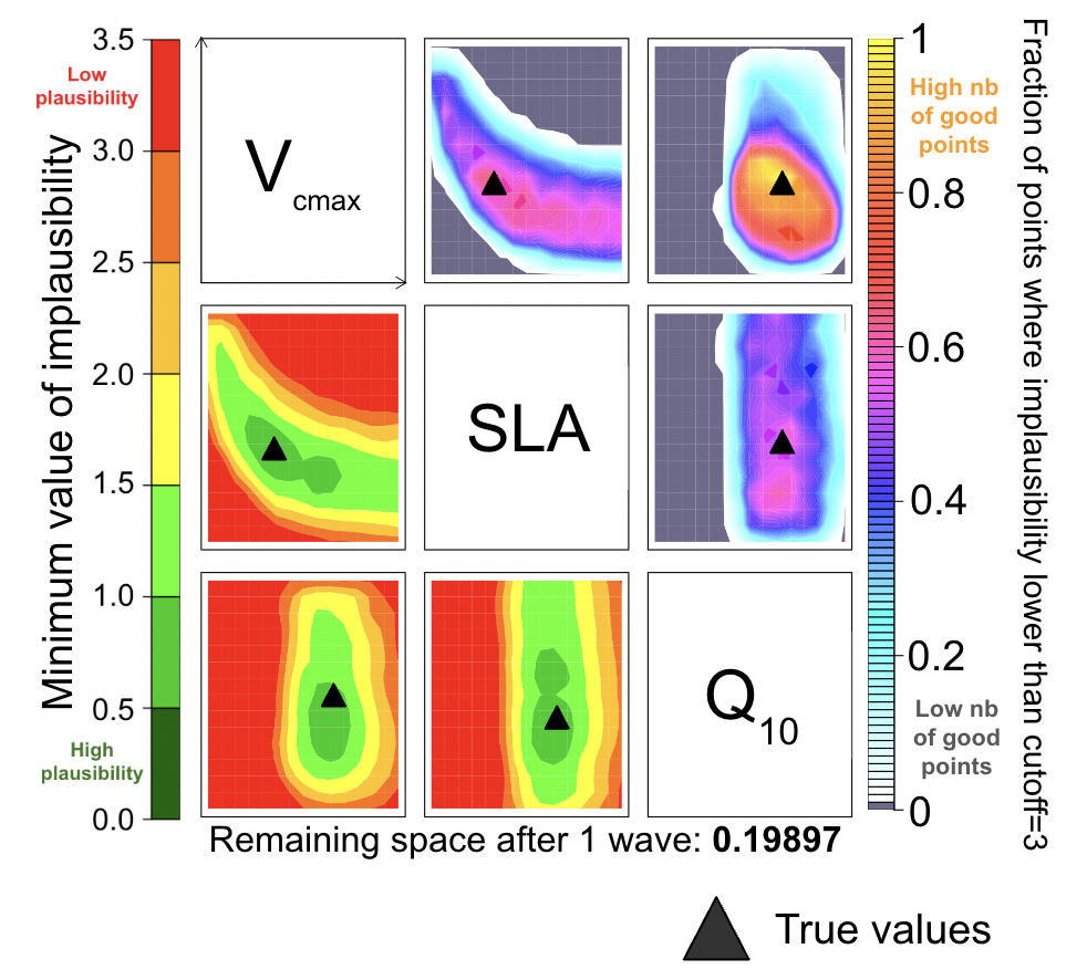
source: Raoult et al. (2024)

Another approach explored during CLARION, is the 4DEnVar technique - a way to use ensembles to get information about the gradient of the cost function, thereby the bypassing the need for the hard to derive/maintain tangent linear/adjoint model or the inprecise finite-different approach.

Novel datasets

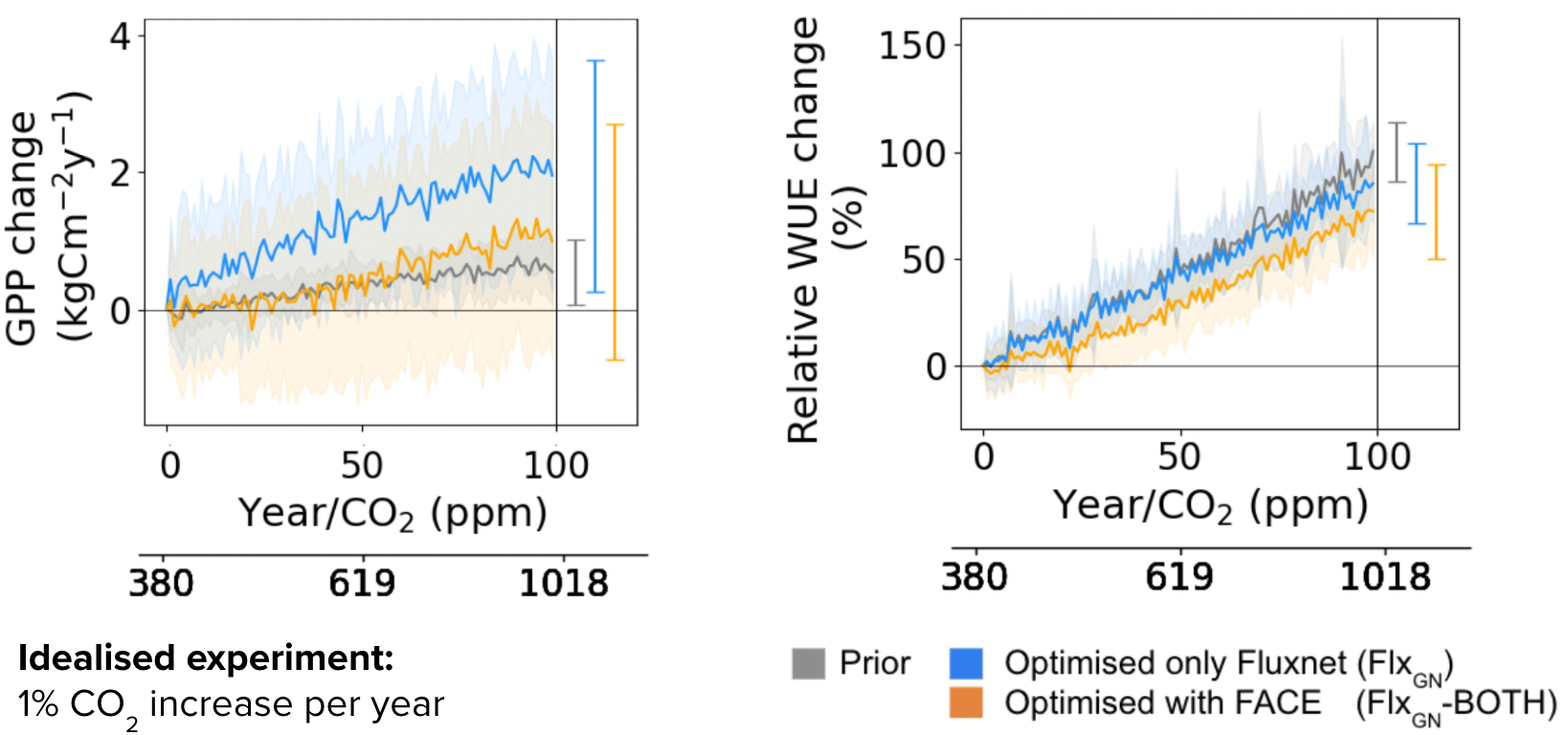
Parameters of land surface models are often calibrated against carbon flux data collected on sites from the FLUXNET network. However, optimising against present-day observations does not automatically give us confidence in future projections of the model, given that environmental conditions are likely to shift compared to the present day. Manipulation experiments give us a unique look into how the ecosystem may respond to future environmental changes. One such type of manipulation experiment, the Free Air CO2 Enrichment (FACE) experiment, provides a unique opportunity to assess vegetation response to increasing CO$_2$ by providing data under ambient and elevated CO$_2$ conditions. Therefore, to better capture the ecosystem response to increased CO$_2$, we add the data from two FACE sites to our optimisations, in addition to the FLUXNET data. When using data from both CO$_2$ conditions of FACE, we find that we are able to improve the magnitude of modelled productivity under both conditions - which allows us to gain extra confidence in the model simulations using this set of parameters.

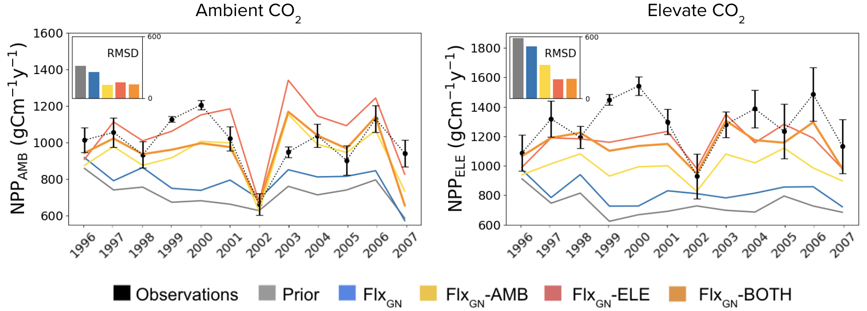
source: Raoult et al. (2024)

Constraining future projections

A parameter perturbation experiment using the UK LSM (JULES) found that projected CO2 change (ΔCO2) by the end of the century varied linearly with Topt — the optimal photosynthesis temperature parameter. a) Varying Topt within its range of uncertainty resulted in a spread of responses larger than that found running the model under different climate scenarios and across different models. b) Combining the relationship between Topt and ΔCO2 with constraints on Topt found by calibrating JULES against in situ daily data, we form an emergent constraint, narrowing the model’s plausible range of climate-carbon cycle feedbacks — with the projected ΔCO2 peaking at 496.5±91 instead of 606.6±128 ppmv.

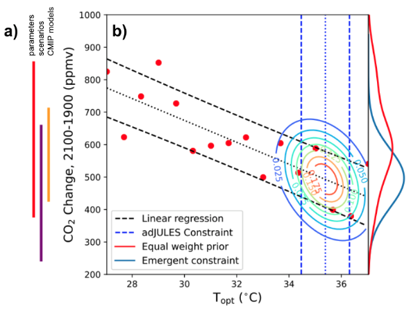
source: Raoult et al. (2023)

Below is another example showing how reduce parameter uncertainty after an optimisation can be fed into constrained climate predictions. Here we should how parameters calibrated in the FACE experiment against both ambient and elevate CO$_2$ conditions give a different trajectory to the default model parameters. Since the calibrated parameters are better able to capture the plant response under different CO$_2$ conditions, we have an increased confidence in their predictions.

source: Raoult et al. (2024)